Getting Started

Installation

Installing Gurobi

AstroQ relies on the Gurobi optimization software to efficiently solve large matrix equations. Follow these steps to install and set up Gurobi:

Create an Account on Gurobi’s registration site. Select that you are an “Academic,” type in your home institution, and submit the form via “Access Now.” You will receive an email to complete the registration.

Download Gurobi for your OS from this download page. Follow the instructions to run the installer file.

Request an Academic License from your user portal while connected to a university network. You want the ‘Named-User Academic License,’ which has a one-year lifetime. At the end of the year, you can obtain a new license easily within your account (and for free) as long as you have maintained your academic status.
Retrieve the License by running the command given in the popup window in a shell. It should look like:
$ grbgetkey 253e22f3...
This command will download a file called gurobi.lic to your machine.
Define the GRB_LICENSE_FILE environment variable by adding the following to your shell profile file:
export GRB_LICENSE_FILE=/path/to/gurobi.lic

Installing AstroQ

We recommend installing AstroQ within a new Anaconda environment. To do so, clone the AstroQ Github repository and run the following commands in the top-level directory:

$ conda env create --name astroq --file environment.yml
$ conda activate astroq

Then install the package:

$ pip install -e .

Installation Test

Run pytest from your terminal to execute a suite of tests verifying that the installation was successful:

$ pytest -v

This may take a few minutes on the first run. The desired result is that all tests pass successfully. However, if you do not have token access to the KPF-CC database, then the test_prep will fail.

Required Files

AstroQ requires six files to run. All example file paths are relative the astroq project directory.

config.ini - Contains configuration information for the AstroQ run.

Example: examples/hello_world/2018B/2018-08-05/band1/config.ini
allocation.csv - Contains information about the nights and times when the telescope is available for observation. It must contain appropriate column headers:
- start
- end
Times are in format “YYYY-MM-DDTHH:MM”

Example: examples/hello_world/2018B/2018-08-05/band1/allocation.csv: (first 5 rows shown):

start

stop

2018-08-05T10:27

2018-08-05T15:07

2018-08-05T05:47

2018-08-05T10:27

2018-08-06T06:30

2018-08-06T08:33

2018-08-06T05:46

2018-08-06T06:30

request.csv - Contains information about the targets and their observational strategies. It must contain appropriate column headers.

unique_id - A unique identifier for the target.
starname - The human-readable name of the target.
program_code - The program code of the target.
ra - The right ascension of the target.
dec - The declination of the target.
exptime - The exposure time of the target.
n_exp - The number of exposures of the target.
n_intra_max - The desired number of visits within a night.
n_intra_min - The acceptable number of visits within a night.
tau_intra - The minimum time (hours) between visits of the target within a night.
n_inter_max - The maximum number of unique nights to observe the target.
tau_inter - The minimum time (days) between unique night observations of the target.
minimum_elevation - The minimum elevation (degrees) of the target.
minimum_moon_separation - The minimum separation (degrees) between the target and the moon.

More columns may be added as needed for your queue (e.g. observational parameters like proper motions, magnitudes, temperatures, etc.) but these are optional record keeping columns.

Example examples/hello_world/2018B/2018-08-05/band1/request.csv:

unique_id	starname	program_code	ra	dec	exptime	n_exp	n_intra_max	n_intra_min	tau_intra	tau_inter	n_inter_max	gaia_id	teff	jmag	gmag	pmra	pmdec	epoch	minimum_elevation	minimum_moon_separation	weather_band_1	weather_band_2	weather_band_3	inactive
e1	HIP1532	U001	4.773176618436250	-9.964852409	360	2	1	1	0	1	20	DR3_2428162410789155328	5000	7.376	9.316666	-36.325	-301.491	2000	33.0	33.0	TRUE	TRUE	TRUE	FALSE
e2	TOI-1670	U002	259.0173367	72.16115935	1200	1	1	1	0	1	30	DR2_1651911084230149248	6200	8.968	9.823196	-6.007	4.923	2000	33.0	33.0	TRUE	TRUE	TRUE	FALSE
e3	191939	U003	302.02397977674000	66.85057684	300	1	1	1	0	25	5	DR3_2248126315275354496	5000	7.597	8.782845	150.194	-63.988	2000	33.0	33.0	TRUE	TRUE	TRUE	FALSE
e4	HAT-P-11	U004	297.7093637403900	48.080861497360000	700	1	1	1	0	2	22	DR3_2086512227851023872	6000	7.608	9.158262	126.095	232.726	2000	33.0	33.0	TRUE	TRUE	TRUE	FALSE
e5	KELT-2	U005	92.66393860111000	30.957142614630000	240	1	1	1	0	1	30	DR3_3438059369839738624	8000	7.669	8.59387	16.726	-2.155	2000	33.0	33.0	TRUE	TRUE	TRUE	FALSE
e6	WASP-107	U006	188.3868505	-10.14617377	450	1	1	1	0	1	10	DR3_3578638842054261248	6000	9.378	11.183329	-96.665	-9.372	2000	33.0	33.0	TRUE	TRUE	TRUE	FALSE
e7	Kepler-10	U007	285.67942245537700	50.24130600481640	50	1	4	2	1	5	30	DR3_2132155017099178624	5000	9.889	10.920031	-18.483	41.382	2000	33.0	33.0	TRUE	TRUE	TRUE	FALSE
e8	55Cnc	U008	133.1492129350180	28.330820831797200	300	1	2	2	2	1	5	DR3_704967037090946688	4000	4.59	5.732681	-485.681	-233.517	2000	33.0	33.0	TRUE	TRUE	TRUE	FALSE
e9	219134	U009	348.3207290015030	57.16835661767190	60	3	1	1	0	1	30	DR3_2009481748875806976	5000	3.86	5.231896	2074.414	294.452	2000	33.0	33.0	TRUE	TRUE	TRUE	FALSE
e10	51Pegasi	U010	344.3665854	20.768832511140000	10	1	1	1	0	1	10	DR3_2835207319109249920	5678	4.66	5.283212	207.328	61.164	2000	33.0	33.0	TRUE	TRUE	TRUE	TRUE
e11	KIC8006161	U010	344.3665854	20.768832511140000	10	1	1	1	0	1	10	DR3_2835207319109249920	5678	4.66	5.283212	207.328	61.164	2000	33.0	33.0	TRUE	TRUE	TRUE	FALSE

past.csv - Contains information about the past history of observations. While it may be blank, it must contain appropriate column headers:

id - the unique identifier for the target.
target - the human-readable name of the target.
semid - the program code of the target.
exposure_start_time_UT - exposure start in UT (legacy column name exposure_start_time is still accepted).
exposure_start_time_local - optional; wall time from UTCoffset when exporting from the OB database.
exposure_time - the recorded duration of the exposure.
NightOf - optional YYYY-MM-DD observing-night label: local calendar date of the most recent sunset at the observatory (from config observatory) before the exposure. Groups pre-midnight and post-midnight data on the same night. If omitted, it is computed when past history is loaded (sunset if the site resolves in astroplan, else a local-noon night boundary).

Example examples/hello_world/2018B/2018-08-05/band1/past.csv:

id	target	semid	timestamp	exposure_start_time_UT	exposure_start_time_local	exposure_time	NightOf	observer	comment
e10	51Pegasi	U010	2018-08-02T05:49:15	2018-08-02T05:44:15	2018-08-01 19:44:15	180	2018-08-01	JackL	Hello World simulated observation
e2	TOI-1670	U002	2018-08-02T20:33:28	2018-08-02T20:28:28	2018-08-02 10:28:28	150	2018-08-01	JackL	Hello World simulated observation
e2	TOI-1670	U002	2018-08-03T20:33:28	2018-08-03T20:31:03	2018-08-03 10:31:03	150	2018-08-02	JackL	Hello World simulated observation
e8	55Cnc	U008	2018-08-02T01:25:13	2018-08-02T01:20:13	2018-08-01 15:20:13	120	2018-07-31	JackL	Hello World simulated observation
e8	55Cnc	U008	2018-08-03T01:25:13	2018-08-03T01:22:18	2018-08-02 15:22:18	120	2018-08-01	JackL	Hello World simulated observation
e6	WASP-107	U006	2018-08-25T06:05:09	2018-08-02T06:00:09	2018-08-01 20:00:09	180	2018-08-01	JackL	Hello World simulated observation

programs.csv - Contains information the awarded time to each program. Useful for plotting later. While it may be blank, it must contain appropriate column headers:
- program - the program code.
- hours - the hours of awarded time to the program.
- nights - the number of nights awarded to the program.
Example examples/hello_world/2018B/2018-08-05/band1/programs.csv:

program

hours

nights

U001

1.0

1.0

U002

1.0

1.0

U003

1.0

1.0

U004

1.0

1.0

U005

1.0

1.0

U006

1.0

1.0

U007

1.0

1.0

U008

1.0

1.0

U009

1.0

1.0

U010

1.0

1.0
custom.csv - Contains information about the specific time windows when targets may be observed. While it may be blank, it must contain appropriate column headers:
- unique_id - the unique identifier for the target.
- starname - the human-readable name of the target.
- start - the start time of the time window.
- stop - the stop time of the time window.
Times are in format “YYYY-MM-DD HH:MM”
Example examples/hello_world/2018B/2018-08-05/band1/custom.csv:

unique_id

starname

start

stop

e1

HIP1532

2018-10-01 00:00

2018-10-30 00:00

e1

HIP1532

2018-08-01 00:00

2018-08-15 00:00

The kpfcc subcommand of prep (see below) compiles and prepares all of these necessary files for the KPF-CC program specifically. Use of this command requires token access to the KPF-CC database. If you are using AstroQ for a different facility, then you must prepare these files through your own means. Feel free to write your own “prep” command to automate the process.

It is strongly recommended that you create the following folder structure for your AstroQ project:

<upstream path>/<semester>/<date>/<band>/

<upstream path> is the path to the top-level directory of your AstroQ project.
<semester> is the semester ID of your project (e.g. 2025B).
<date> is the date you are generating the schedule (e.g. 2025-08-01).
<band> is the weather band number (use band1 if you not interested in multiple bands).

For example, if your upstream path is /Desktop/, your semester is 2025B, your date is 2025-08-01, and your band is 1, then your folder structure should be: /Desktop/2025B/2025-08-01/band1/

In this folder structure, you should place (or automate the creation of) the necessary files above to run AstroQ. We recommend a new folder for every run, so as to create a history of schedules. You may further create additional weather bands within the date level. Each band should get its own copy of all files.

Command Line Interface

Test your installation further by running some of the commands below. We will use AstroQ’s command line interface to mock up a toy observing schedule. After performing the steps in the Installation section, you should have access to the astroq binary at the command line. If not, ensure that you have run pip install -e . in the top-level directory of the repository.

Let’s see which subcommands are available using astroq --help:

$ usage: astroq [-h] [-V] {bench,plot,kpfcc_prep,webapp,plan-semester,plan-night,compare} ...

    AstroQ: Optimized observation scheduling

    optional arguments:
    -h, --help            show this help message and exit
    -V, --version         Print version number and exit.

    subcommands:
    {bench,plot,prep,webapp,plan-semester,plan-night,compare}

The AstroQ command-line interface provides the following subcommands:

bench - Runs the benchmark test. Here you can compare your computer’s performance with the AstroQ benchmark from our paper, Lubin et al. 2025.
prep - Compile and prepare all necessary files. For the KPFCC program, there is an additional subcommand kpfcc. Note that if you are building a queue for a different facility, you will have to build your own subcommand.
webapp - Launch web app to view interactive plots for a given solution of AstroQ.
plan-semester - Solve for the optimal semester-long schedule, determining what stars to observe on what nights. This is the heart of AstroQ.
plan-night - Solve for the optimal slew path using the TTP package.
compare - Compare two AstroQ solutions.

Below are more detailed explanations of these commands and their outputs.

Hello World Example

To create your mock observing schedule, let’s run the hello world example. Here we have supplied the necessary files. We will create a schedule for the first night when we have the telescope, 2024-08-02, as specified in the config file. Navigate to your AstroQ/ directory and then run:

$ astroq plan-semester -cf examples/hello_world/config_hello_world.ini

Let’s take a look at the outputs produced:

$ ls -ltr examples/hello_world/2018B/2018-08-05/band1/outputs

    -rw-r--r--@ 1 jack  staff    3153 Oct 29 12:15 semester_plan.csv
    -rw-r--r--@ 1 jack  staff  230542 Oct 29 12:15 serialized_outputs_dense_v1.csv
    -rw-r--r--@ 1 jack  staff  253640 Oct 29 12:15 serialized_outputs_dense_v2.csv
    -rw-r--r--@ 1 jack  staff     346 Oct 29 12:15 runReport.txt
    -rw-r--r--@ 1 jack  staff     873 Oct 29 12:15 request_selected.csv
    -rw-r--r--@ 1 jack  staff  244512 Oct 29 12:15 semester_planner.h5

semester_plan.csv contains the id, day, slot and name of the scheduled observations. sorted by target name. See example:

r

d

s

name

e1

4

62

HIP1532

e1

5

66

HIP1532

e1

8

65

HIP1532

e1

12

61

HIP1532

e1

13

82

HIP1532

e1

61

77

HIP1532

e1

63

76

HIP1532

e1

64

77

HIP1532

e1

86

67

HIP1532

e1

87

67

HIP1532

e2

4

36

TOI-1670

e2

5

35

TOI-1670

e2

8

41

TOI-1670

serialized_outputs_dense_v1.csv contains the same information, but now all slots, even those not scheduled to have an observation are included, and it is ordered by time. See example:

d

s

r

name

0

0

0

1

0

2

0

3

0

4

0

5

0

6

0

7

0

8

0

9

0

10

0

11

0

12

0

13

0

14

…

…

…

…

4

62

e2

HIP1532

4

63
serialized_outputs_dense_v2.csv is identical to serialized_outputs_dense_v1.csv, but now slots that cannot be filled for all stars (like sky brightness or telescope allocation, are denoted with an “X”). See example:

d

s

r

name

0

0

X

0

1

X

0

2

X

0

3

X

0

4

X

0

5

X

0

6

X

0

7

X

0

8

X

0

9

X

0

10

X

0

11

X

0

12

X

…

…

…

…

4

62

e2

HIP1532

4

63

runReport.txt: contains some basic statistics about the fullness of the schedule. See example (note, this schedule is not supposed to be a good one!):

Stats for Round1
------------------------------------------------------
N slots in semester:26496
N available slots:2874
N starting slots scheduled: 183
N reserved slots: 26
N total slots scheduled: 209
N slots left empty: 2665
N slots requested (total): 807
Utilization (% of available slots): 7.272%
Utilization (% of requested slots): 25.898%

request_selected.csv: contains a copy of the request.csv file but only for the targets that were selected to be observed.:
semester_planner.h5: is a serialized and compressed version of the splan object used for scheduling. This will be used later in the webapp/plotting routines and serves as a record of the schedule inputs/outputs.

Now that we have the stars to be observed each night of the semester, let’s determine the optimal ordering of the stars selected for tonight, mimizing slew times, to generate a night plan:

$ astroq plan-night -cf examples/hello_world/config_hello_world.ini

Here are the new files in examples/hello_world/outputs/:

-rw-r--r--@ 1 jack  staff     447 Oct 29 13:36 ttp_prepared.csv
-rw-r--r--@ 1 jack  staff     433 Oct 29 13:36 TTPstatistics.txt
-rw-r--r--@ 1 jack  staff     158 Oct 29 13:36 ObserveOrder_2018-08-05.txt
-rw-r--r--@ 1 jack  staff    1157 Oct 29 13:36 script_2018-08-05_nominal.txt
-rw-r--r--@ 1 jack  staff   16080 Oct 29 13:36 night_planner.h5

ttp_prepared.csv is the input to the TTP solver. It contains the target information in the format required by the TTP solver. See example and the TTP repository for more info:

Starname

RA

Dec

Exposure Time

Exposures Per Visit

Visits In Night

Intra_Night_Cadence

Priority

First Available

Last Available

e1

4.77317661843625

-9.964852409

360

2

1

0

10

2018-08-05 10:20

2018-08-05 15:00

e2

259.0173367

72.16115935

1200

1

1

0

10

2018-08-05 05:50

2018-08-05 08:50

e7

285.679422455377

50.2413060048164

50

1

4

1

10

2018-08-05 05:50

2018-08-05 12:20

e9

348.320729001503

57.1683566176719

60

3

1

0

10

2018-08-05 08:40

2018-08-05 15:00

TTPstatistics.txt contains some basic statistics about the TTP solution. See example:

Stats for TTP Solution
------------------------------------
    Model ran for 0.05 seconds
    Observations Requested: 7
    Observations Scheduled: 7
Maximum Observations Bound: 1
------------------------------------
Observing Duration (min): 560.00
Time Spent Exposing (min): 40.57
    Time Spent Idle (min): 510.51
Time Spent Slewing (min): 8.92
Minimum Slew Bound (min): 4.17
------------------------------------

ObserveOrder_2018-08-05.txt the timestamps at which each star is set to be observed. See example:

unique_id

Target

StartExposure

e2

TOI-1670

05:47

e7

Kepler-10

06:07

e7

Kepler-10

07:07

e7

Kepler-10

08:47

e9

219134

08:49

e1

HIP1532

11:41

e7

Kepler-10

11:59
script_2018-08-05_nominal.txt is a backwards compatible file in the style of the old HIRES queue night plans.
night_planner.h5: a serialized and compressed version of the night planner object use to schedule. This will be used later in the webapp/plotting routines.

Now we can launch the webapp to view the schedule. This will launch on a local server at http://localhost:50001. When it launches, append “/2018B/2018-08-05/band1/admin” to the URL to view the admin page. Check out and familiarize yourself with the various figures and reports.

$ astroq webapp -up examples/hello_world/

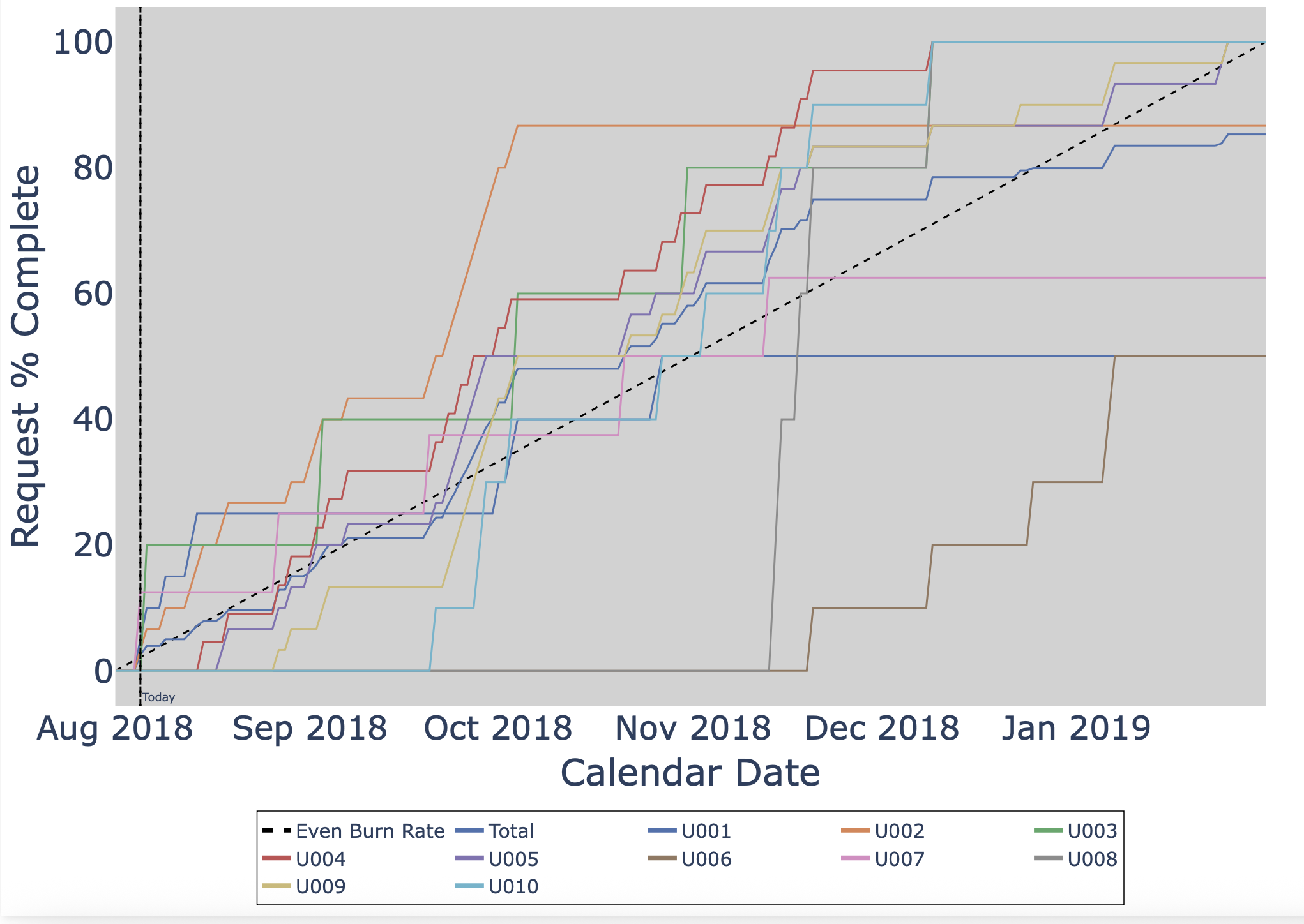
Scrolling down a bit, you should see the “Cumulative Observation Function (COF)” plot which describes the completion rate of each program as a function of time:

Scrolling down a bit, you should see the “birdseye” plot of the schedule look something like this:

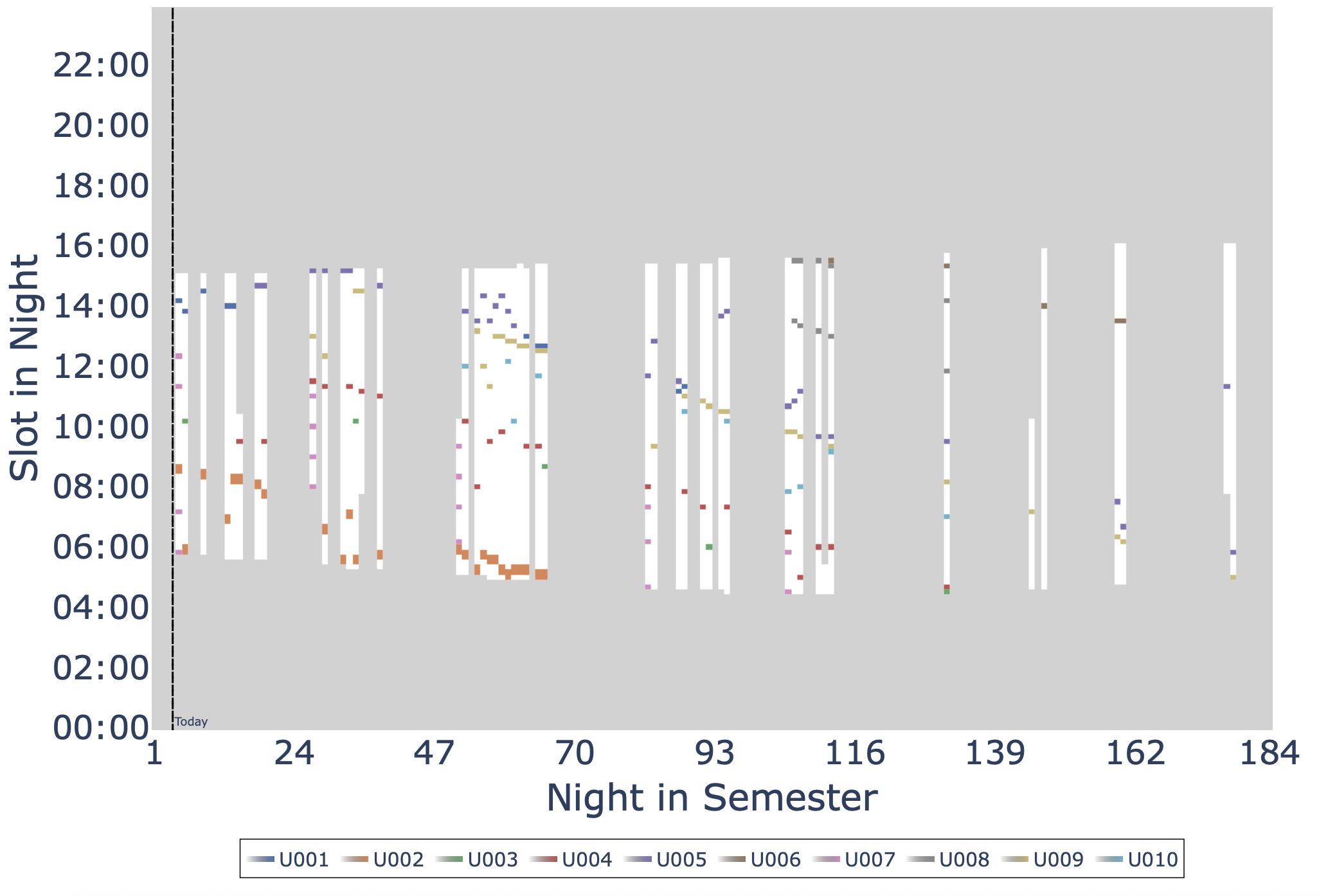
Notice that two program perform poorly, U001 and U006. This is entirely explainable and stems from the fact that the requests in these programs are infeasible. For example, let’s investigate U006’s target, WASP-107. First displaying all the slots that are available for observations this semester:

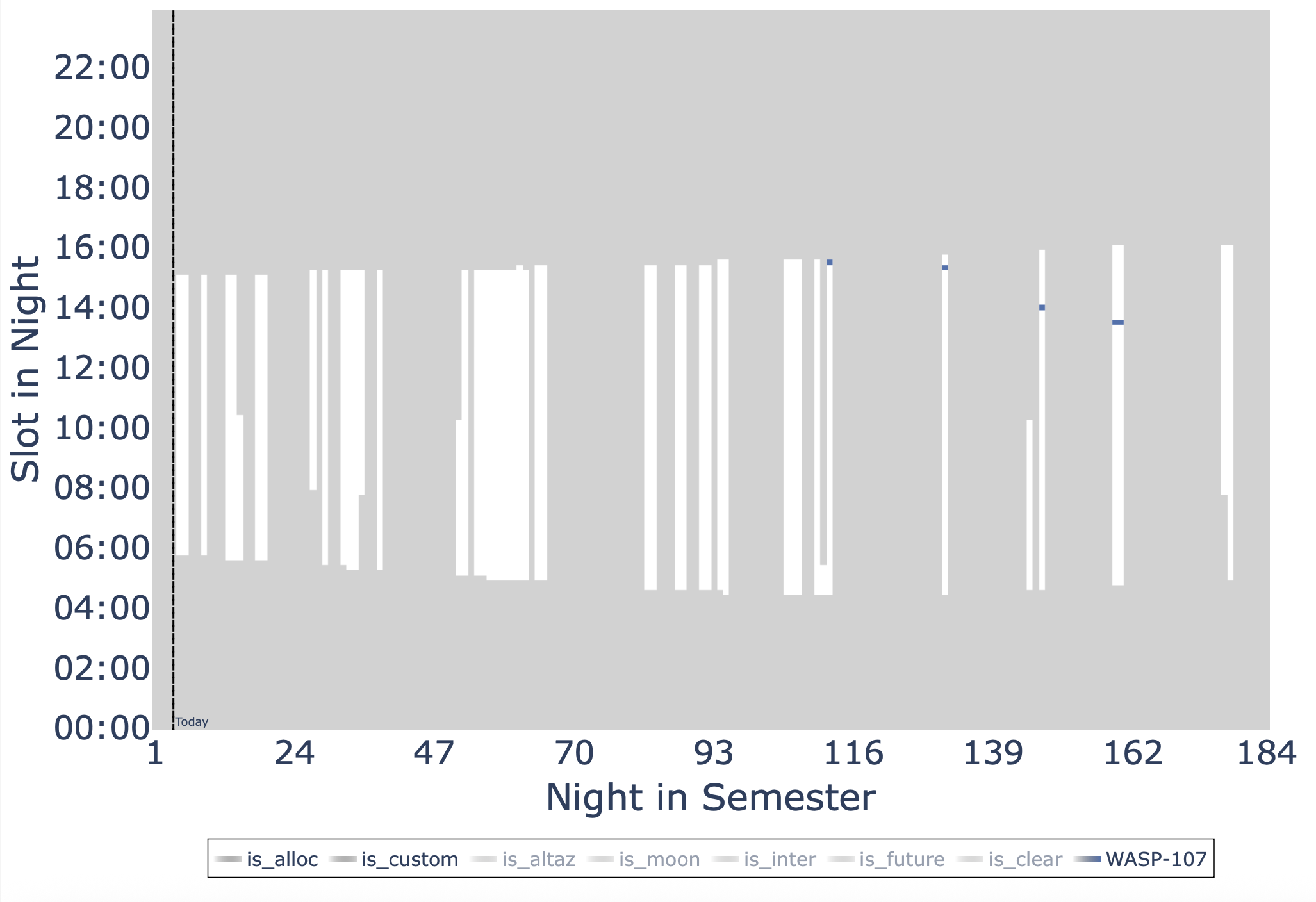
This shows there is lots of available time to schedule the target. So why isn’t it getting scheduled more? Turning on some of the individual constraint maps reveals the problem. First we turn on the is_altaz, which blocks out the times that are not available for scheduling this target due to the natural seasonality of the star and the pointing limits of the telescope:

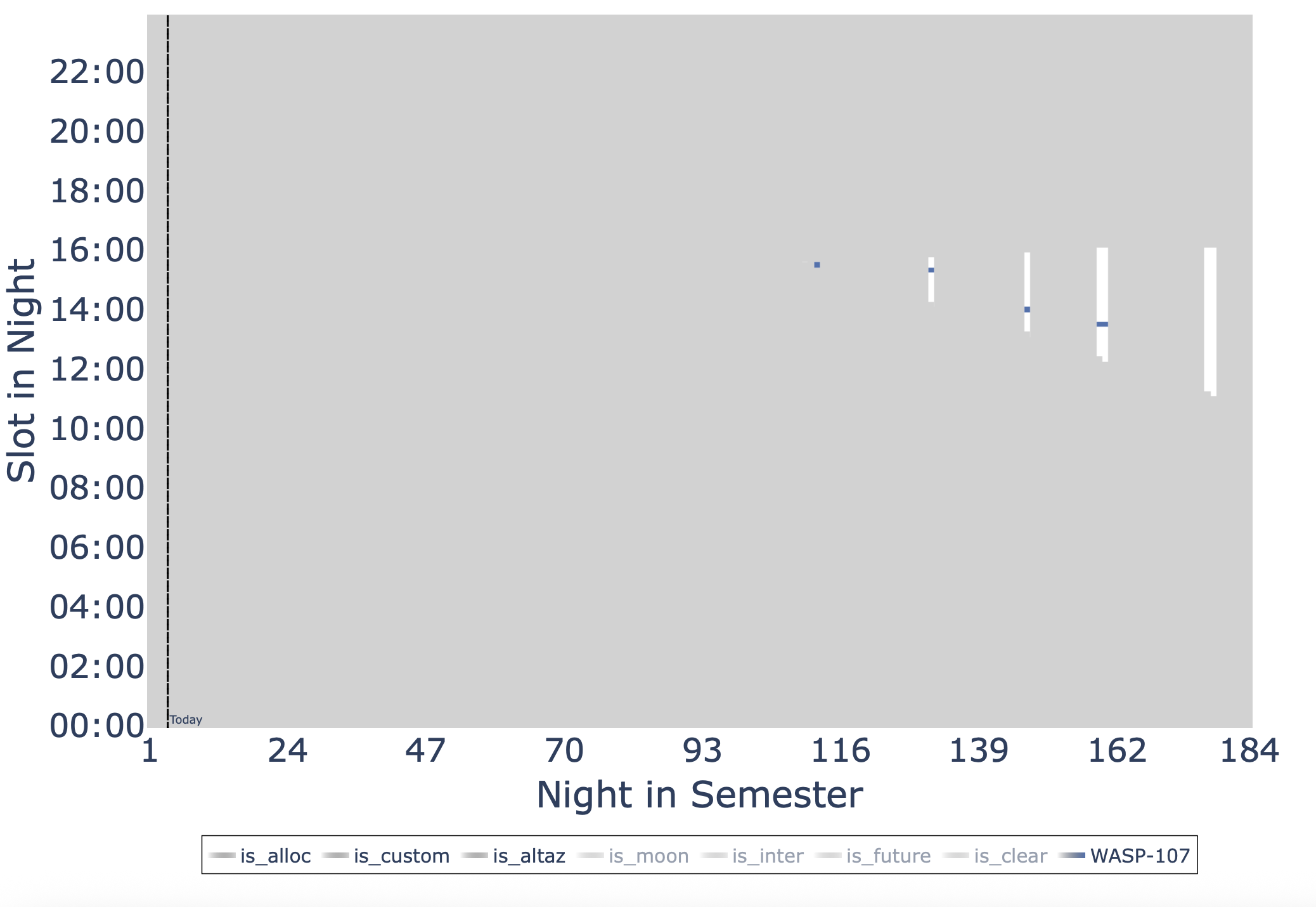
Immediately we see that the vast majority of our allocated time is not ammenable to observing this target. But what about those last two days, why isn’t the target scheduled then? We can further turn on the is_moon, which blocks out the times that are not available for scheduling this target due to the moon’s position in the sky and we see that this is the cause of conflict:

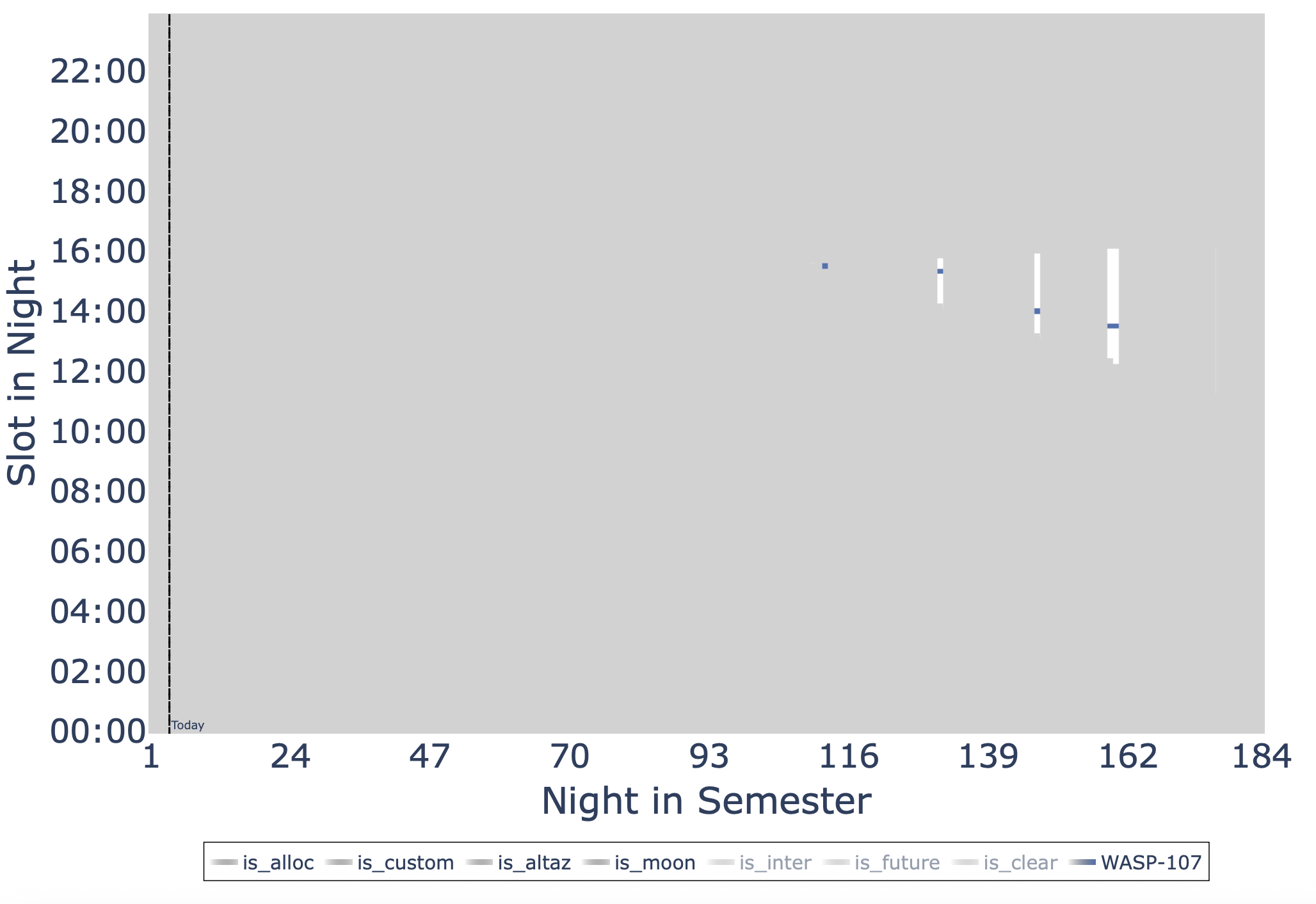
Now we can feel confident that AstroQ is scheduling this target as often as is feasible. The request itself is infeasible, thus the low completion rate. U001’s HIP1532 target is amenable to observations all semester, but it has a custom map that severly restricts when it can be observed, hence a low completion rate. These tools allow us the really dive into any target and understand why it is or is not being scheduled.

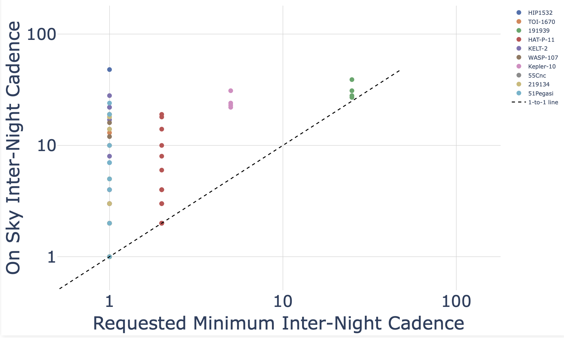
Looking at some additional plots, we track the on-sky cadence vs the requested cadence. We don’t want to violate the PI’s desired minimum cadence so all dots on this plot should be above the dashed line, which, is confirmed:

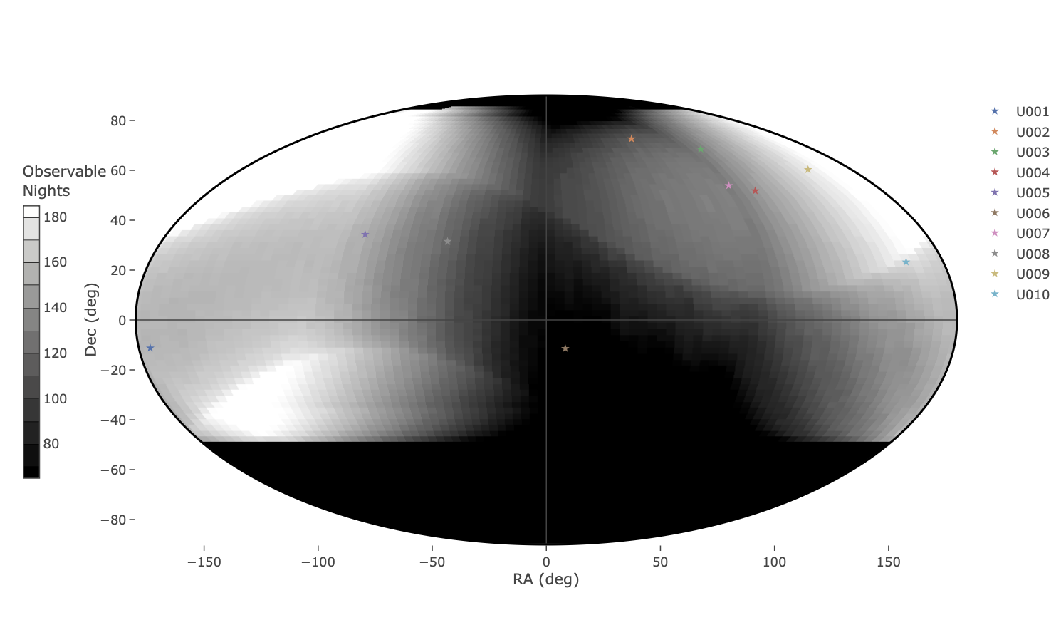
Lastly, we look at the distribution of the targets across the sky. Against the grayscale heatmap, we can get a sense for how many nights in the semester a given location on the sky is observable, imagining we had the telescope all night every night. Here we can quickly see that WASP-107 is in a dark region of the sky, meaning it is not amenable to many observations in the semester. Couple that with the fact that we don’t actually have all night every night to observe, this target is severely limited in its observability and hence has the low completion, which we walked through above. This grayscale map captures the intricate pointing limits of the K1 telescope easily.

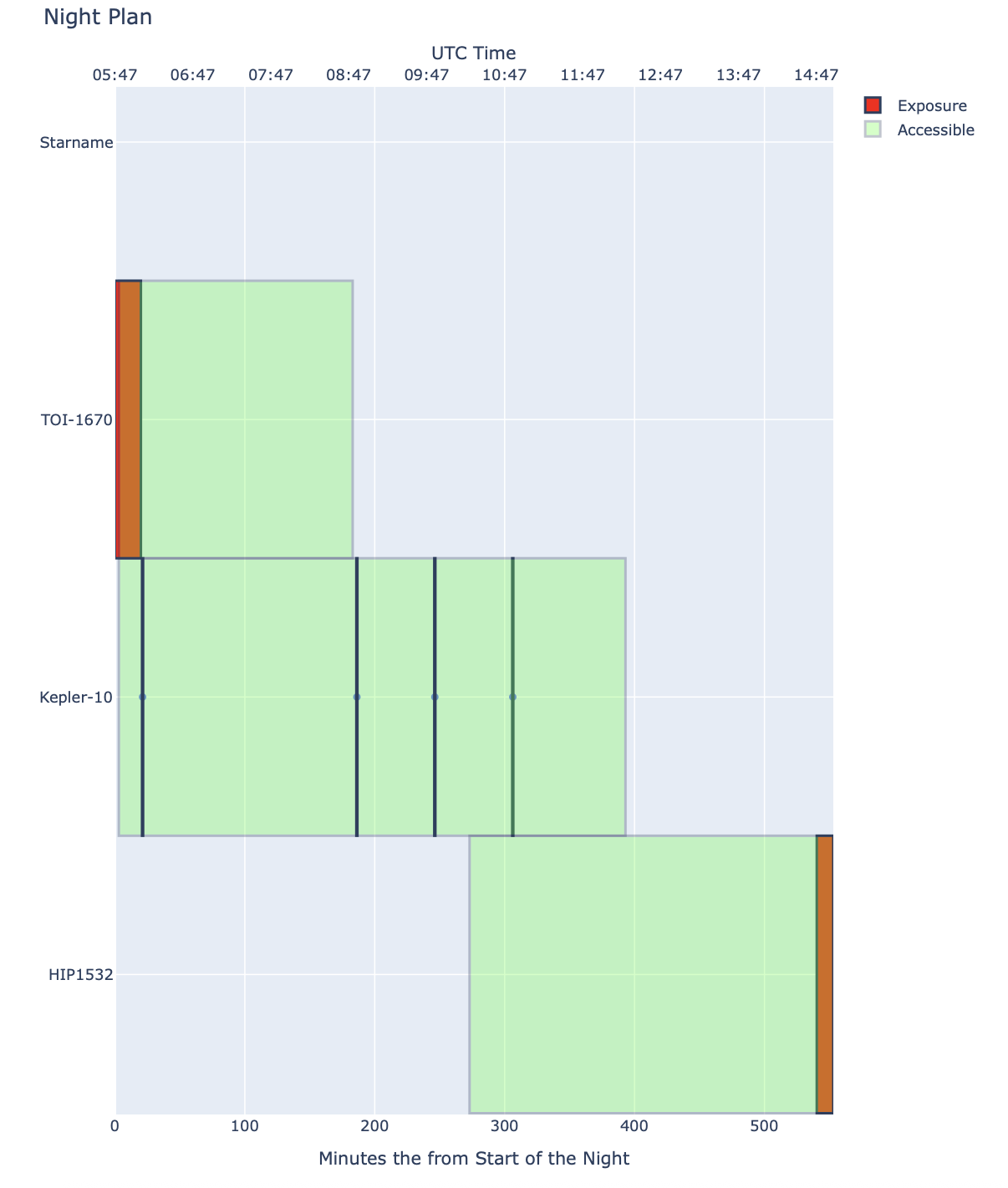
Next we can investigate the plan for tonight. After the the slew path in minimized through the TTP solver, we have a suite of plots availabe to us for insight. First we look at the “ladder” plot. The observations are ordered in time from top to bottom. Green bars indicate the spans of time when the target is observable (above pointing limits), and the red bars indicate the times when we are set to observe the target. We can easily see the plan for the night, and see how tight or loose the windows are to observe a particular target.

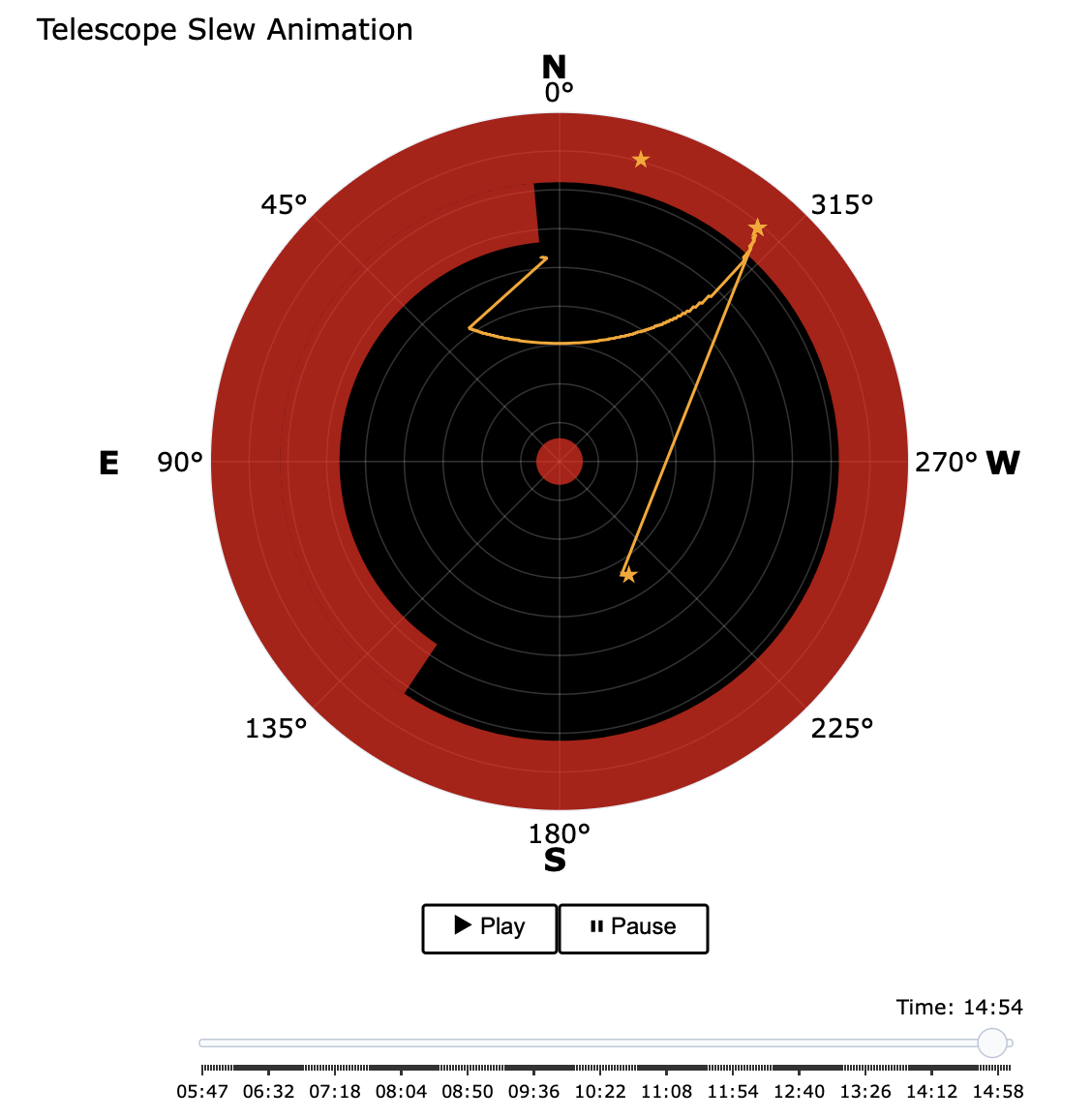
Then we have the slew path animation (screenshot below). This is a polar plot of the telescope’s slew path with an orange line showing the path of the telescope over the night as the defined optimal path. The red regions are below/above telescope pointing limits and are unique to K1 telescope. The slider at the bottom allows us to select a time in the night and see where we are and where we are going next.

The Hello World Example is an easy model to solve. It only has 10 requests, with a total of 282 observations to schedule across and entire 6 month semester…a human could do this easily. In terms of model size, it is only 4598 rows by 8285 columns with 65656 nonzeros.

Try something a bit more complex by running our benchmark test. This is a realistic semester model scheduling 200 requests with programs of different observational strategies inspired by real observing programs. This model is 56009 rows by 329369 columns with 3820641 nonzeros, significantly bigger and not human-solvable.

$ astroq bench -cf examples/bench/config_benchmark.ini -ns 12

The inputs and expected outputs are well defined in our paper, compare your computer’s performance to ours! See Lubin et al. 2025.

start	stop
2018-08-05T10:27	2018-08-05T15:07
2018-08-05T05:47	2018-08-05T10:27
2018-08-06T06:30	2018-08-06T08:33
2018-08-06T05:46	2018-08-06T06:30

program	hours	nights
U001	1.0	1.0
U002	1.0	1.0
U003	1.0	1.0
U004	1.0	1.0
U005	1.0	1.0
U006	1.0	1.0
U007	1.0	1.0
U008	1.0	1.0
U009	1.0	1.0
U010	1.0	1.0

unique_id	starname	start	stop
e1	HIP1532	2018-10-01 00:00	2018-10-30 00:00
e1	HIP1532	2018-08-01 00:00	2018-08-15 00:00

d	s	r	name
0	0
0	1
0	2
0	3
0	4
0	5
0	6
0	7
0	8
0	9
0	10
0	11
0	12
0	13
0	14
…	…	…	…
4	62	e2	HIP1532
4	63